TOF-SANS Working Group: Difference between revisions
From canSAS
No edit summary |
No edit summary |
||
| Line 28: | Line 28: | ||
Few other open issues not covered with the information above: | Few other open issues not covered with the information above: | ||
* Spacings of resolution curve still needs to be defined (in principle it could match the Q spacings of the I(Q)) | |||
* Think about whether to use anything more advanced that Trapezium Rule for the integrations. | |||
* Think about Q resolution for 2d data! | |||
Revision as of 20:52, 20 March 2024
Members
- Andrew Jackson (ESS)
- Anna Sokolova (ANSTO)
- Sebastian Jaksch (ESS)
- Judith Houston (ESS)
- Adrian Rennie (Uppsala)
- Wojciech Potrzebowski (ESS)
News/Status
- Working group formed at canSAS-XI in Freising
- The workshop about TOF resolution was held in March 2021 (online): https://indico.esss.lu.se/event/2506/
Generic resolution function
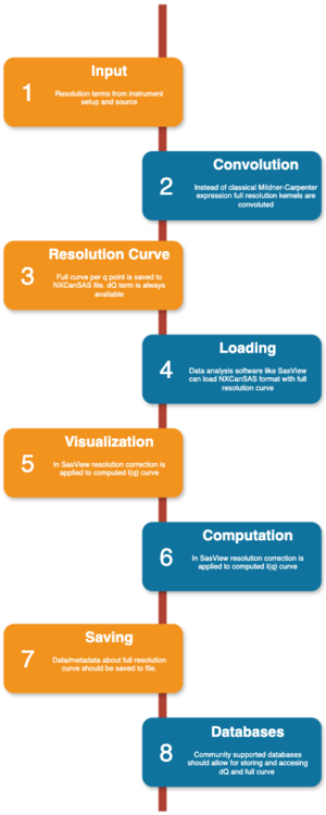
A workflow for utilizing the full resolution curve is shown in figure 1.
In order to avoid repetitions and keep the message coherent, bellow I provided mostly the collection of relevant links and current status (March 2024).
- Input data consists of instrumental parameters and shapes of corresponding terms contributing to the resolution function. Please check https://github.com/scipp/esssans/issues/111 for more details
- Convolution. Following developments in GRASP individual resolution kernels are convoluted rather than collapsed to a single number (as classically has been done with Milldner-Carpenter equation). Please review Jupyter notebook on how this can be potentially done https://github.com/scipp/esssans/files/14509637/checkbox-convolution.ipynb.zip
- Resolution curve. The full-resolution curves (defined per q points) are saved to NXCanSAS file. Anticipates entries are /entry/data/q/resolutions and /entry/data/q/resolutions_descriptions. dQ as a single number should always be provided.
- Loading. NXCanSAS files with resolution functions need to be loaded by the analysis software. It will require development in SasView.
- Visualization. Majority of users will probably apply resolution as it is. It may however be useful to be able to plot individual resolution curves and for example, compare it with Gaussian estimates. There may also be some option for changing sampling. This part needs to be defined and developed.
- Computation. Proof-of-concept of applying full resolution curve has been demonstrated using SasView: https://github.com/SasView/sasview/blob/generic_resolution/notebooks/GenericResolutionPOC.ipynb. (Also https://github.com/SasView/sasview/issues/1497)
- Saving. The information about the full resolution curve should be carried on as metadata or the report. It needs to be established
- Databases. It would also be useful if community supported databases can consume this information (both dQ and full description).
Few other open issues not covered with the information above:
- Spacings of resolution curve still needs to be defined (in principle it could match the Q spacings of the I(Q))
- Think about whether to use anything more advanced that Trapezium Rule for the integrations.
- Think about Q resolution for 2d data!
